Visualizing the Stability of 2D Point Sets from Dimensionality Reduction Techniques
C. Reinbold1, A. Kumpf1, R. Westermann1
1Computer Graphics & Visualization Group, Technische Universität München, Germany
Abstract
We use k-order Voronoi diagrams to assess the stability of k-neighborhoods in ensembles of 2D point sets, and apply it to analyze the robustness of a dimensionality reduction technique to variations in its input configurations. To measure the stability of k-neighborhoods over the ensemble, we use cells in the k-order Voronoi diagrams, and consider the smallest coverings of corresponding points in all point sets to identify coherent point-subsets with similar neighborhood relations. We further introduce a pairwise similarity measure for point sets, which is used to select a subset of representative ensemble members via the PageRank algorithm as an indicator of an individual member's value. The stability information is embedded into the k-order Voronoi diagrams of the representative ensemble members to emphasize coherent point-subsets and simultaneously indicate how stable they lie together in all point sets. We use the proposed technique for visualizing the robustness of t-SNE and multi-dimensional scaling applied to high-dimensional data in neural network layers and multi-parameter cloud simulations.
Associated publications
Visualizing the Stability of 2D Point Sets from Dimensionality Reduction Techniques
C. Reinbold, A. Kumpf, R. Westermann
Please note: The following preprint summarizes the main ideas of our work. Please refer to the final version for detailed explanations and analysis. It is published by Computer Graphics Forum and is available here.
Method Overview

Let X be a finite set of n entities in some multi-dimensional coordinate or parameter space. Our method analyzes an ensemble E of embeddings of X into the 2D plane. Each embedding is an ordered 2D point set P of cardinality n. Points in different ensemble members that have the same index refer to the same entity.
To analyze whether certain subgroups of points are stably connected—using a suitable neighborhood relation—across all ensemble members, we introduce the depicted pipeline. In general, for a certain subgroup of size k, all n over k available subgroups need to be tested. As this is intractable, we utilize k-order Voronoi diagrams—computed in step (a)—to reduce this number to O(kn) many k-neighborhoods. The k-order Voronoi diagrams provide topological information that is used to assemble neighborhoods of fixed size k into subgroups of arbitrary size. The geometric structure of these diagrams is further used to visualize simultaneously the stability information that is obtained from it and a 2D embedding of X.
In step (b), the stability of each k-neighborhood is assessed using minimum covering circles of the corresponding point set in all other ensemble members. In this way, multiple stability values are obtained for each neighborhood. These values are finally aggregated into a single value that quantifies the overall stability of a neighborhood in the ensemble (step (c)).
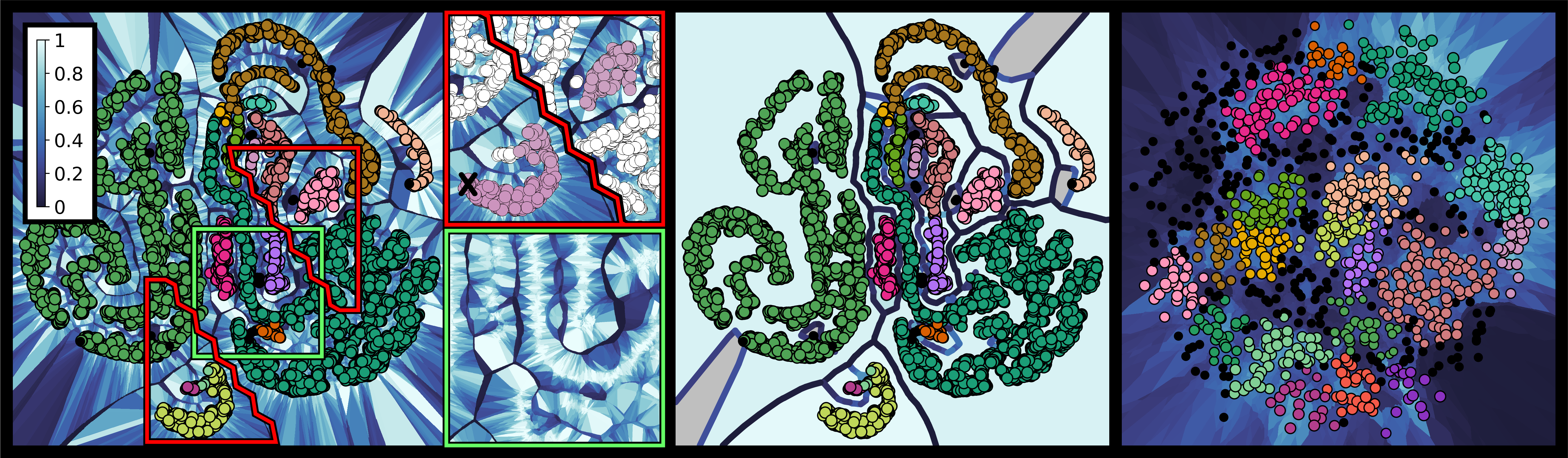
To ease the interpretation, an abstract visualization is provided in which the information is condensed. Therefore, the major information regarding stable subgroups and their relations to each other is extracted by clustering the k-order Voronoi diagrams (step (d)). A region's stability is mapped to its background color, and ridges between these regions are colored to indicate how strongly adjacent subgroups are separated. The visualization allows to immediately identify points which are connected via k-neighborhoods of locally high stability.
For each point set P, distinct plots can be generated. Many of these plots carry similar information, in particular regarding the stable regions. Building upon a pairwise similarity matrix that is computed in step (e), a small set of representative plots is finally selected in step (f). These plots carry most of the stability information, and they are used to embed the stability information into the 2D domain. The plots of any ensemble member reveal the agreement of the member to the derived stability information.
Stability analysis
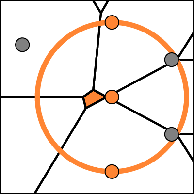
Our notion of stability is based on how well neighborhoods are preserved in different point sets: Given a k-subset V of points in one point set, how large is the spread of these points in all other point sets. This is determined by computing the smallest possible disks that cover the points in V in the other sets. These disks may also cover points not being part of V, indicating that additional points interfere with the neighborhood relationship. The stability value stab(V,P) of V with respect to P is then computed as the ratio between k and the number of points covered by the disk. Consider P containing the gray and orange points as in the figure, and V containing the three orange points. Then, stab(V,P) evaluates to 3/5, since the cardinality of V is 3 and the smallest disk covering V contains 5 points.
Voronoi Diagrams
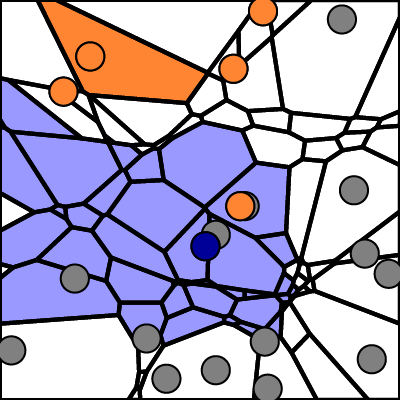
The subsets V that are considered in the stability analysis are computed from the higher order Voronoi diagrams. We sample all k-nearest neighborhoods induced by every possible location in 2D space. When grouping all 2D locations according to their k-nearest neighborhoods, a partition of the 2D space into a finite number of (possibly unbounded) convex regions is obtaind. These regions are called Voronoi cells. A many-to-many correspondence between cells and points is established by relating a cell to each of its k-nearest points (see figure). The partition is called the k-order Voronoi diagram of the given point set and extends the well known (1-order) Voronoi diagram. The computation of k-order Voronoi diagrams is tractable for modest values of k, with run-time complexity O(k2n log n), and yields O(kn) neighborhoods [1].
Clustering and Visualizing Stable Subgroups of Points
The interpretation of higher order Voronoi diagrams is challenging. To ease the interpretation of k-order Voronoi diagrams, density aware clustering is used (step (d)). The approach builds upon the observation that in k-order Voronoi diagrams, when their cells are colored according to the stability of neighborhoods, regions packed with stable, connected components are often separated by instable bands (see teaser–left). By means of clustering, these components are extracted and translated to subgroups of stable points. Hence, considerably larger stable areas than k-neighborhoods can be identified and put into releation to each other. Two points are located in the same cluster if they are part of the same stable submanifold, whereas a submanifold is considered stable if it occurs in most of the point sets of the ensemble. The topological structure of the submanifold is outlined by ridges (see teaser–middle).
Clustering of Voronoi Cells
From a k-order Voronoi diagram, enriched by stability information, connected areas of locally high stability can be emphasized by arranging the Voronoi cells in a hierarchical manner. For this, we utilized concepts from persistent homology [2, 3]. Let λ with 0 ≤ λ ≤ 1 be an arbitrary threshold. For a selected λ, the superlevel set L+(λ) is the set of all Voronoi cells with a stability value greater or equal to λ. The superlevel set is comprised of a set of connected components Comp(λ). When λ is decreased towards 0, these components merge until one connected component remains. By relating a component to all components that have been merged to form it, a tree of components is generated that serves the desired hierarchical representation. For instance, the depicted Voronoi diagram yields the hierarchical representation that is shown by Dendrogram (1).
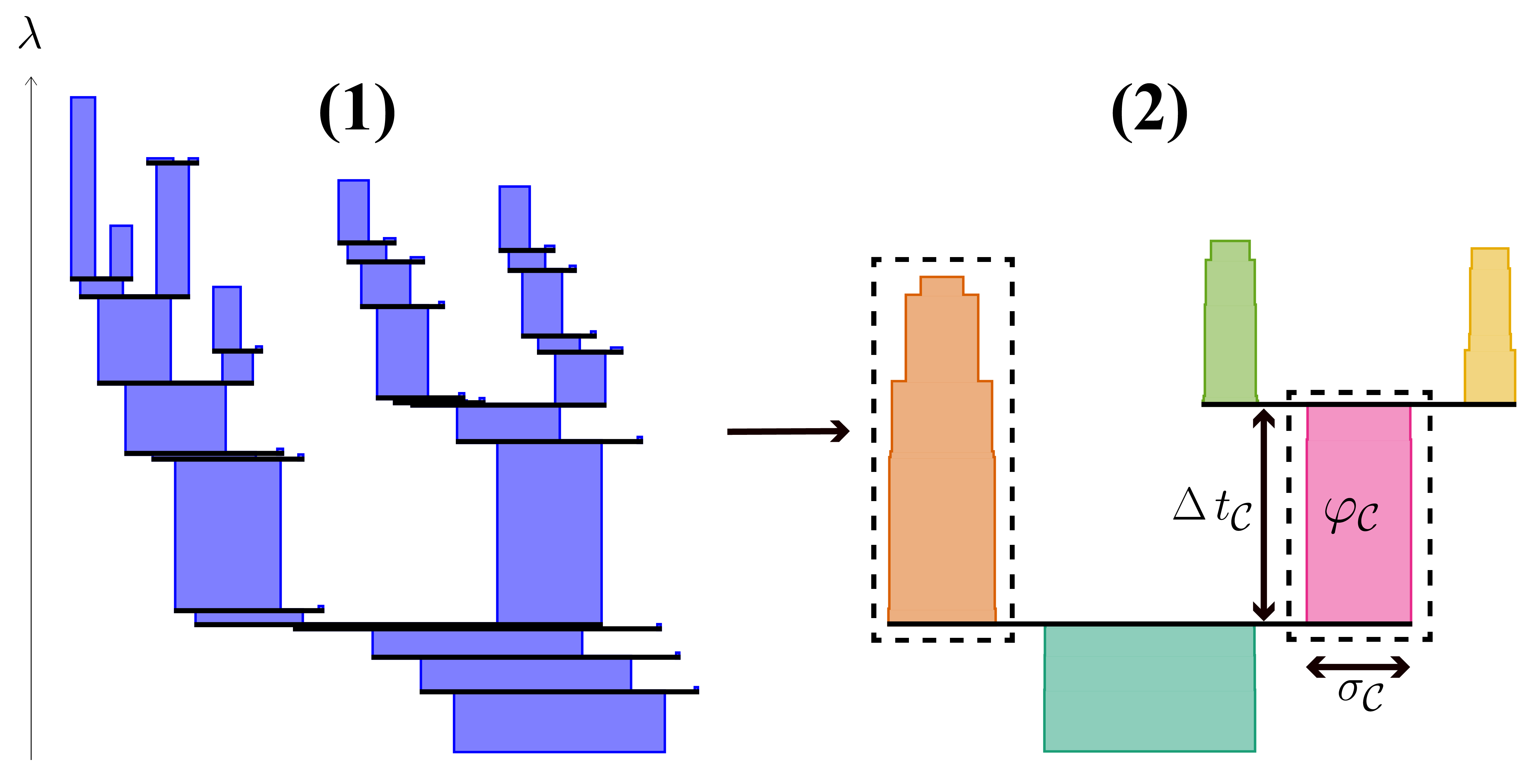
We utilize the same concept as used in the clustering technique HDBSCAN [4] in order to extract prominent clusters from the hierarchical representation. HDBSCAN slices the merge tree at different depths such that components which persist for an extended duration before merging into another one are kept intact. In order to detect persistent components, sufficiently small components and their merge events are dropped beforehand. In doing so, the method becomes robust against noise. Additionally, we introduce a significance term σC as well as a persistence term φC for each connected component C. Significance of a component roughly represents the amount of points described by that cell. Its persistence is computed by integrating the significance over the components lifetime ΔtC. The box width displayed in the Dendrograms encodes signficance whereas box area encodes persistence.
Finally, a set of disjoint connected components are selected such that the sum of their persistence values becomes maximal. The selected set represents the final clustering of the Voronoi cells, of which some may not be covered and thus considered noise. In Dendrogram (2), the selected components are framed by dashes. They represent the upper and lower half of cells in the sample Voronoi diagram respectively. The instable cells forming the horizontal subdivison are considered noise.
Point Clusters
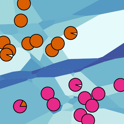
To relate the Voronoi cell clusters to the initial point set, these clusters are interpreted as fuzzy point clusters, and hard point clusters are derived by a fix assignment of points to their most likely cluster. Since an initial point can be part of many equally stable neighborhoods, it contributes fractions to each cell C the point is related to. A Voronoi cell can now be related to a fuzzy point cluster by gathering the contributions from points contained in its k-nearest neighborhood. A Voronoi cell cluster may be interpreted as a fuzzy point cluster by adding up all contributions of the cells contained in the cluster. When applying the process to the sample Voronoi diagram together with its Voronoi Cell clustering, the depicted fuzzy point clustering is obtained. Defuzzying yields the expected clustering that separates points contributing to the upper and lower Voronoi cells respectively.
Abstract visualization
We propose an abstract visualization of k-order Voronoi diagrams. In addition to showing the point set in a scatterplot, points in different clusters as well as points deemed noise are separated via ridges. Ridge color encodes how strongly clusters are separated. The background color of a cluster encodes a weighted average of stability values over all cells assigned to the cluster.
Selection of Representative Point Sets
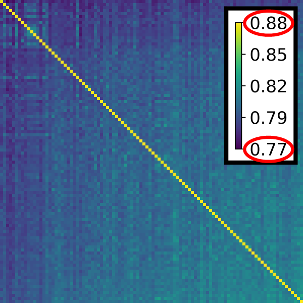
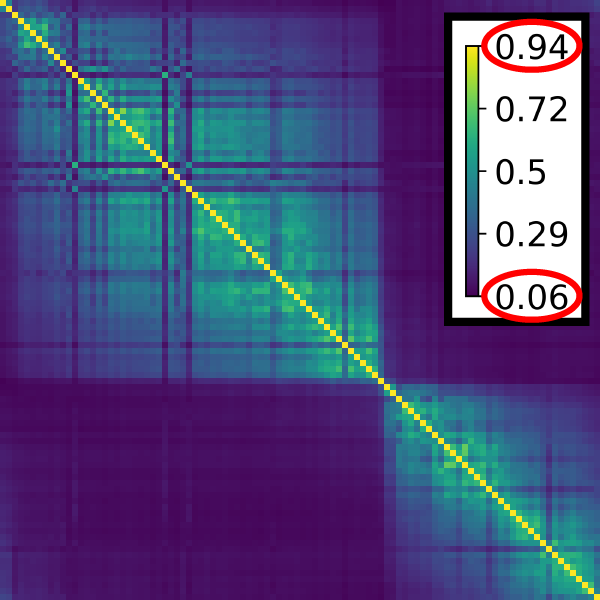
Since a single plot for each ensemble member would overburden the visualization, we guide the user’s selection process of viewing certain point sets in step (f) by computing a pairwise similarity matrix in step (e) of the pipeline. The pairwise similarity between point sets P,Q encodes how well the k-neighborhoods arising in Q are preserved in the point set P. Exemplary similarity matrices for two different point set ensembles are shown on the right. In order to extract clusters of similar point sets in the ensemble, matrix seriation [5] is used to sort columns and rows such that hidden patterns become apparent.We utilize the two rank ellipse seriation of Chen [6] for identifying blocks of point sets as shown in the right matrix. When the blocks are identified, for each block a representative is picked that is determined by the highest score when applying the PageRank algorithm [7].
(Some) Results
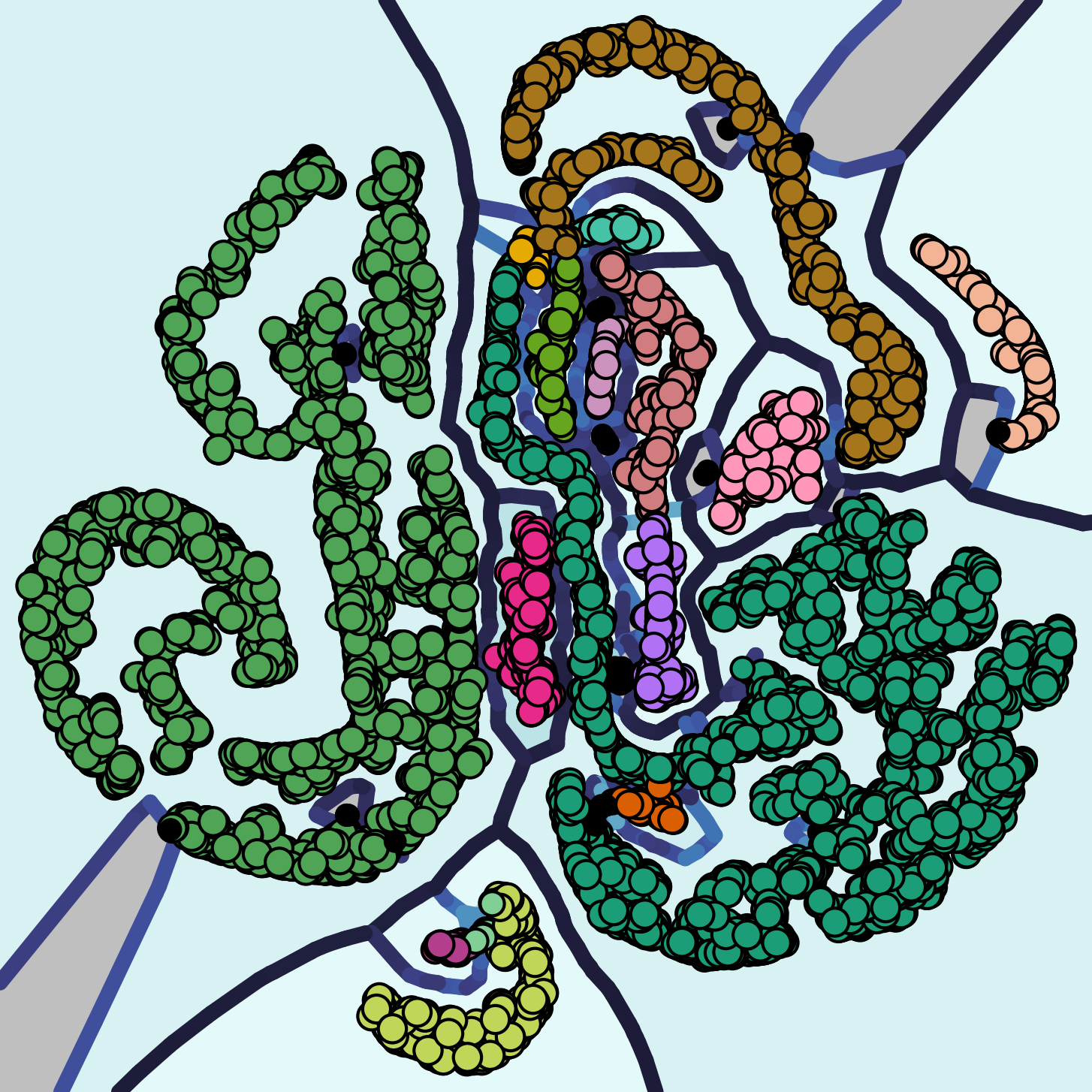
The generated plots allow us to consistently detect misplaced points in the selected point set, i.e. points that could not be placed appropriately by t-SNE. Those appear as noise points colored in black. Additionally, not all bands and vicinities formed by t-SNE are meaningful. Note that we are able to point out misleading structures such as the small attachment of the crescent at the bottom of the figure. In most point sets of the ensemble, this attachment is detached from the crescent.
It is common knowlegde that for t-SNE projections, "distances between clusters might not mean anything" [8]. We give meaning to distances by drawing separating ridges between clusters located next to each other by chance (see separated bands at the center) and omitting them where clusters regularly are placed next to each other (see entangled band structures at the bottom right).
References
- Der-Tsai Lee: On k-Nearest Neighbor Voronoi Diagrams in the Plane. IEEE Transactions on Computers C-31, 6 (June 1982), 478–487. doi: 10.1109/TC.1982.1676031.
- Herbert Edelsbrunner and John Harer: Persistent Homology — a Survey. Contemporary mathematics 453 (2008), 257–282.
- Herbert Edelsbrunner and John Harer: Computational topology: an introduction. American Mathematical Soc., 2010.
- Ricardo J.G.B. Campello, Davoud Moulavi and Jörg Sander: Density-Based Clustering Based on Hierarchical Density Estimates. In Advances in Knowledge Discovery and Data Mining (Berlin, Heidelberg, 2013), Pei J., Tseng V. S., Cao L., Motoda H., Xu G., (Eds.), Springer Berlin Heidelberg, pp. 160–172. doi: 10.1007/978-3-642-37456-2_14.
- Michael Behrisch, Benjamin Bach, Nathalie Henry Riche, Tobias Schreck and Jean‐Daniel Fekete: Matrix Reordering Methods for Table and Network Visualization. Computer Graphics Forum 35, 3 (2016), 693–716. doi: 10.1111/cgf.12935.
- Chun-Houh Chen: Generalized Association Plots: Information Visualization via Iteratively Generated Correlation Matrices. Statistica Sinica 12, 1 (2002), 7–29.
- Sergey Brin and Lawrence Page: The anatomy of a large-scale hypertextual Web search engine. Computer Networks and ISDN Systems 30, 1 (1998), 107 – 117. Proceedings of the Seventh International World Wide Web Conference. doi: 10.1016/S0169-7552(98)00110-X.
- Martin Wattenberg and Fernanda Viégas and Ian Johnson: How to Use t-SNE Effectively, Distill (2016). doi: 10.23915/distill.00002